ST3002 Assignment Correlation and Regression

Correlation and Regression

Part 1 — Correlation in Research

For this section, refer to the following article from the Walden Library:

References

Slavic, D., Jakovljevic, D. K., Zubnar, A., Tapavicki, B., Aleksandric, T., & Drapsin, M. (2019). Effects of different types of training on weight loss. Medicinski Pregled/Medical Review, 72(9/10), 272–279. https://doi.org/10.2298/MPNS1910272S

All articles are available in full text in the Walden Library, which you may search by title or DOI. Be sure to provide an explanation for each of your answers and include supporting evidence from the text and/or Learning Resources.

Write responses to address the following in paragraph form by inserting your answers directly beneath the questions.

On page 277 (Journal page number), there are six scatter plots. Use these scatter plots to answer the following questions

1. Rank the six correlations provided from lowest correlation to highest correlation. Include a 2- to 3-sentence explanation as to why you ranked these the way you did.

The following is the ranking of the six correlations, ordered from lowest to highest.

1. Fat mass (r = 0.334)
2. Height (r = 0.360)
3. Body weight (r = 0.442)
4. Femur breadth (r = 0.535)
5. Skeletal muscle mass (r = 0.553)
6. Fat-free mass (r = 0.563)

Explanation

The ranks are statistically based on the correlation coefficient (r), which indicates the relationship between resting metabolic rate (RMR) and the various anthropometrics. The higher the R-value, the closer the two variables are related. The lowest correlation is with fat mass (r = 0.334), signifying a weak effect. The correlation indicates that femur width and skeletal muscle mass are significantly related to RMR, while fat-free mass is most strongly related (r = 0.563) because lean tissue uses up more energy than fat tissue. Throughout the analysis, the correlation coefficient (r) is found to range from -1 to 1. In statistics, a positive correlation is indicated by a positive value of r, which indicates a positive relationship between variables, meaning that as the value of one variable increases, the other increases as well. If two variables move in opposite directions, then one variable increases as the other variable decreases, there is a negative correlation. An r value close to 0 means it is not related, and if the value close to 1 or -1 means it has a strong positive or negative relationship (Xu et al., 2023). The positive R-value results in this study indicate direct correlations for all anthropometric measurements to RMR.

2. Choose ONE of the six graphs and compute the r-squared value. Interpret this value in regard to variation.

Calculation

R²= (0.553)²=0.306

Interpretation

The 30.63% of RMR variation that can be attributed to skeletal muscle mass shows through the R² value of 0.306. The remaining 69.37% of the variance is from factors not included in skeletal muscle mass, but which have accounted for 30.63% of the variability of RMR.

3. Using the information presented on this page, explain one reason why BMI does not always indicate an individual’s health status (correlation does not imply causation).

BMI does not allow us to see a person’s health, as it equates muscle and fat. The increased muscle mass from athletes’ anaerobic training improves their BMI score. The measurement doesn’t accurately reflect how well balanced an athlete’s body structure and health are, as the higher BMI could be due to increased muscle strength rather than increased weight gain.

Part 2 — Analyzing the Relationships between Health Factors

The following should be based on the data set you created from the larger BODY DATA (ST3001) data set using the instructions provided.

Scatter plots

Replace this text with your Excel output created and explanations using the following instructions:

• BMI and LDL cholesterol levels
  • Create a scatterplot for the data in the BMI and LDL cholesterol columns. Paste it in your report.

The scatterplot visually represents the relationship between BMI (x-axis) and LDL (y-axis) cholesterol.

• Using Excel, calculate the linear correlation between the data in the BMI and LDL cholesterol columns.

Paste your results in your Word document. Explain the mathematical relationship between BMI and LDL cholesterol based on the linear correlation coefficient. Be certain to include comments about the magnitude (strength) and the direction (positive or negative) of the correlation. As BMI increases, what happens to LDL cholesterol?

BMI oppositely correlates with -0.22091 with HDL cholesterol. There is a weak relationship between BMI growth and decreasing HDL cholesterol in the body. As the BMI increases, the level of HDL cholesterol decreases, our results showed. The weak correlation number (close to zero) indicates that BMI is used on its own with a weak correlation with HDL cholesterol level. Several other factors contribute to HDL cholesterol numbers that aren’t known. In the small but not significant association, increasing BMI is associated with a decreasing number of HDL cholesterol levels.

• BMI and HDL cholesterol levels
  • Create a scatterplot for the data in the BMI and HDL cholesterol columns. Paste it in your report.

The scatterplot shows the relationship between BMI and HDL cholesterol.

• Using Excel, calculate the linear correlation between the data in the BMI and HDL cholesterol columns. Paste your results in your Word document.

• Explain the mathematical relationship between BMI and HDL cholesterol based on the linear correlation coefficient. Be certain to include comments about the magnitude (strength) and the direction (positive or negative) of the correlation. As BMI increases, what happens to HDL cholesterol?

The research results reflect that the BMI and HDL are inversely proportional, with the negative value of the slope b1 = -0.5205. The study revealed a negative correlation of -0.5205 between HDL and BMI, showing that with each unit increase in BMI, HDL is expected to decrease by 0.5205 units. Results of the research indicate that the BMI value at 25 (57.5062) and the BMI value at 40 (49.6987) show a continuous downward trend as HDL decreases with increasing BMI. The BMI tends to be higher when the HDL level is lower in the body, and this is a significant health risk.

Simple Linear Regression and Predictions

Replace this text with your Excel output created using the following instructions:

• Using this sample data, perform a linear regression to determine the line of best fit. Use BMI as your x (independent) variable and HDL as your y (response) variable. Use four (4) places after the decimal in your answer. Paste it in your report.

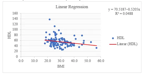
The graph shows a weak negative relationship between BMI and HDL, as indicated by the regression equation y = 70.5187 – 0.5205x.

• What is the equation of the line of best fit (linear regression equation)? Present your answer in y = b_o + b₁x form.

The linear regression equation is given by:

y=b₀+b₁x

From the regression output

• b₀ (Intercept) = 5187
• b₁ (Slope for BMI) = -0.5205

Thus, the equation is

y=70.5187−0.5205x

• What would you predict the HDL would be for a patient with a BMI of 25? Show your calculations.

Substituting x=25 into the equation

y=70.5187−0.5205 (25)

y=70.5187−13.0125

y=57.5062

So, the predicted HDL for a patient with BMI = 25 is 57.5062.

• What would you predict the HDL would be for a patient with a BMI of 40? Show your calculations.

Substituting x=40 into the equation

y=70.5187−0.5205 (40)

y=70.5187−20.82

y= 49.6987

So, the predicted HDL for a patient with BMI = 40 is 49.6987

What effect would you predict BMI would have on HDL levels? Use your computations above to justify your reasoning.

The research results reflect that the BMI and HDL are inversely proportional, with the negative value of the slope b1 = -0.5205. The study revealed a negative correlation of -0.5205 between HDL and BMI, showing that with each unit increase in BMI, HDL is expected to decrease by 0.5205 units. Results of the research indicate that the BMI value at 25 (57.5062) and the BMI value at 40 (49.6987) show a continuous downward trend as HDL decreases with increasing BMI. The BMI tends to be higher when the HDL level is lower in the body, and this is a significant health risk.

Calculate the coefficient of determination (R² value) for this data. What does this tell you about this relationship?

The regression output gave R² = 0.0488, which means that the variability in the HDL level is 4.88% due to BMI. The negative slope value in b₁ = -0.5205 indicates that there is a 0.5205 unit decrease in HDL for every 1 unit increase in BMI. According to the regression findings, patients with a BMI of 25 will have 57.5062 HDL, while those with a BMI of 40 will have 49.6987 HDL in our model. HDL levels are clearly decreasing between BMI 25 and BMI 40. The little predictive power of BMI for measuring HDL levels is shown through the low R² value, as other factors are believed to affect HDL levels, like diet, exercise, genetics, and health conditions. There is a statistical correlation between BMI and HDL, but BMI is not useful as a single measure for estimating HDL in clinical practice.

Multiple Linear Regression

Replace this text with your response to the following:

• Using this sample data, perform a multiple-regression line of best fit using age, systolic blood pressure, and BMI as predictor variables and pulse rate as the response variable. Paste your Excel work in your report.

• What is the equation of the line of best fit? The form of the equation is: Y = b_o + b₁X₁ + b₂X₂ + b₃X₃ (fill in values for b_o, b₁, b₂, and b₃). Round coefficients to three (3) decimal places.

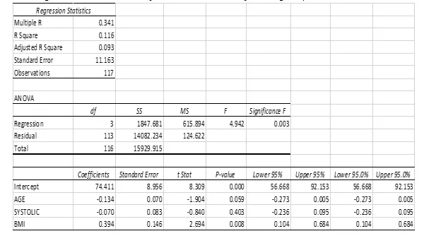
From the Coefficients table:

• Intercept (b0) = 74.411
• AGE (b1) = -0.134
• SYSTOLIC (b2) = -0.070
• BMI (b3) = 0.394

Y = 74.411-0.134X1 -0.070X2 + 0.394X3   

• What would you predict the pulse rate be for a patient with who is 33 years old with a systolic blood pressure of 110 and BMI of 27?

Y= 74.411−0.134 (AGE) −0.070 (SYSTOLIC) +0.394(BMI)

Y=74.411−0.134 (33) −0.070 (110) +0.394(27)

Y= 74.411−4.422−7.7+10.638

Y= 72.927

The predicted pulse rate for a 33-year-old with a systolic blood pressure of 110 and a BMI of 27 is 72.93.

• What is the R² value for this regression? What does it tell you about regression?

            R² values of a regression are used to measure the variation explained by the independent variable(s) from the dependent variable; the scale ranges from 0 to 1. The higher the value, the better the fit (Fey et al., 2022). Although all variables are included in the model, the model accounts for only 11.60% of the variation in pulse rate with age, blood pressure, and BMI; the 88.40% of the rate’s variability due to these three variables is left unaccounted for. The regression model predicted less than a good amount of the changes in pulse rate; over 88% were due to UN modelled details. BMI shows a statistically strong relationship with pulse rate at a high significance level (P-value = 0.008), although the overall model is not very predictive. The results demonstrate that the model has very little predictive ability, as indicated by the value of adjusted R² (0.093). Age, systolic blood pressure, and BMI are attributes that provide some information about pulse rate, te but on their own would not yield statistically significant forecasting results. The results confirm that a full model (medical and daily-life measurements) would foster better predictions.